Cohort Analysis with Python

Using Python to understand user retention is much easier than you might have imagined. All of this can be done with a few libraries. For this tutorial, we will be using Pandas, Matplotlib and Seaborn and Datetime.

You can follow the along in the video to save time if you are in a rush.

You can also follow the code below to ensure that you know how to create the full cohort using Python. Make you change the file path to fit where your file is saved. The full Jupyter notebook is hosted on Github here.

# import libraries 
import pandas as pd
import matplotlib.pyplot as plt
import seaborn as sns 

# load in the data and take a look 
data = pd.read_excel("C:/Users/User/Downloads/Online Retail.xlsx")


#drop rows with no customer ID
data = data.dropna(subset=['CustomerID'])
#create an invoice month
import datetime as dt

#function for month
def get_month(x):
    return dt.datetime(x.year, x.month,1)

#apply the function 
data['InvoiceMonth'] = data['InvoiceDate'].apply(get_month)

#create a column index with the minimum invoice date aka first time customer was acquired
data['Cohort Month'] =  data.groupby('CustomerID')['InvoiceMonth'].transform('min')
data.head(30)

# create a date element function to get a series for subtraction
def get_date_elements(df, column):
    day = df[column].dt.day
    month = df[column].dt.month
    year = df[column].dt.year
    return day, month, year 

# get date elements for our cohort and invoice columns
_,Invoice_month,Invoice_year =  get_date_elements(data,'InvoiceMonth')
_,Cohort_month,Cohort_year =  get_date_elements(data,'Cohort Month')

#create a cohort index 
year_diff = Invoice_year -Cohort_year
month_diff = Invoice_month - Cohort_month
data['CohortIndex'] = year_diff*12+month_diff+1

#count the customer ID by grouping by Cohort Month  and Cohort Index 
cohort_data = data.groupby(['Cohort Month','CohortIndex'])['CustomerID'].apply(pd.Series.nunique).reset_index()

# create a pivot table 
cohort_table = cohort_data.pivot(index='Cohort Month', columns=['CohortIndex'],values='CustomerID')

# change index
cohort_table.index = cohort_table.index.strftime('%B %Y')
#visualize our results in heatmap
plt.figure(figsize=(21,10))
sns.heatmap(cohort_table,annot=True,cmap='Blues')

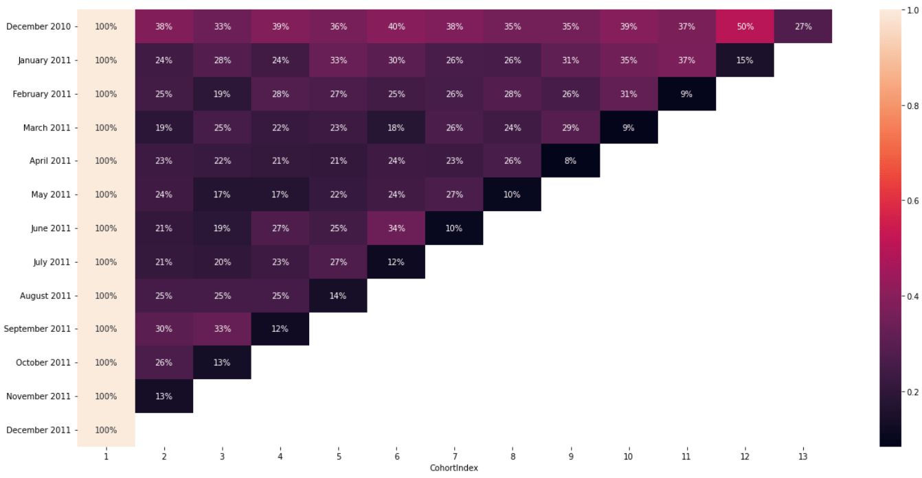
#cohort table for percentage
new_cohort_table = cohort_table.divide(cohort_table.iloc[:,0],axis=0)

#create a percentages visual
plt.figure(figsize=(21,10))
sns.heatmap(new_cohort_table,annot=True,fmt='.0%')