How to Do Data Profiling in Excel?

Making sense of your data with Excel is smart because it’s both powerful and budget-friendly. Data profiling in Excel helps you see what’s in your data, from the good bits to the bits that might need some work. And the best part? Excel is easy to get and often free, so you can dive into your data projects without worrying about the cost. This guide is here to help you get really good at data profiling with Excel, making your data work more effective and insightful.

What is Data Profiling?

Data profiling is the process of examining the data available in an existing database and collecting statistics or informative summaries about that data. The goal of data profiling is to gain a clear understanding of the quality, structure, and challenges of the data before it is used for data projects or analytics.

How to do Data Profiling in Excel: Step-by-Step

Step 1: Import Your Data into Excel

Open Microsoft Excel and load the data into Excel. 

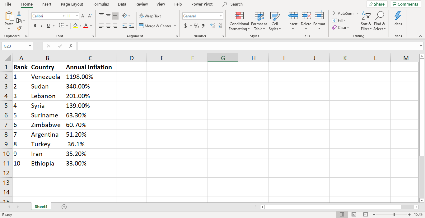
Note: You can go to the “File” menu and select “Open” to open your dataset if it’s already in an Excel file. Alternatively, you can select “Import” if your data is in another format (like CSV or TXT). Ensure that your data is arranged in rows and columns in a tabular format.

Step 2: Use the Power Query Editor

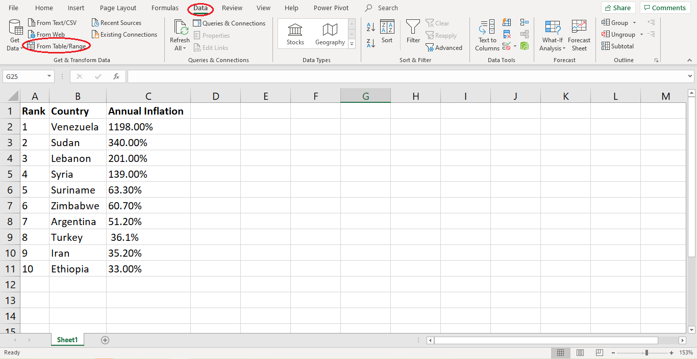
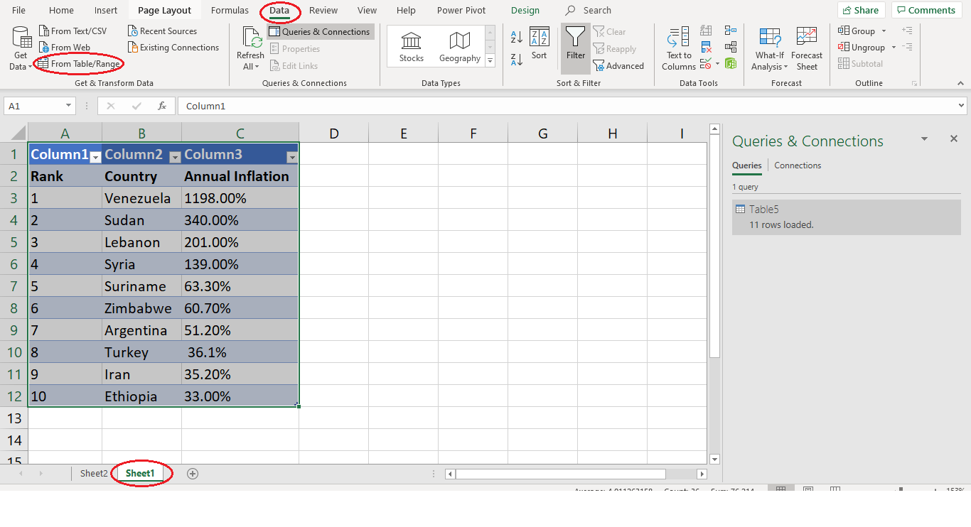
Go to the “Data” tab and select from table range. 

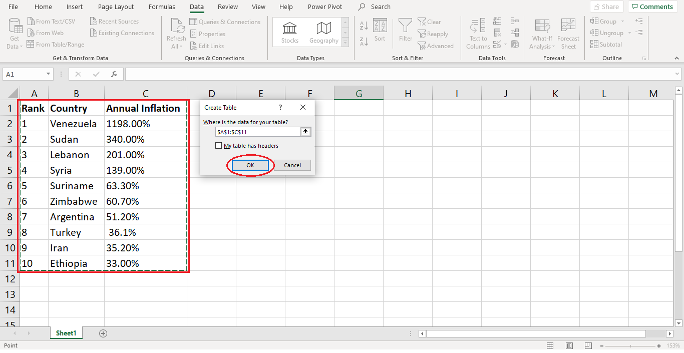
When the Create Table prompt appears, highlight the entire table and click “OK”.

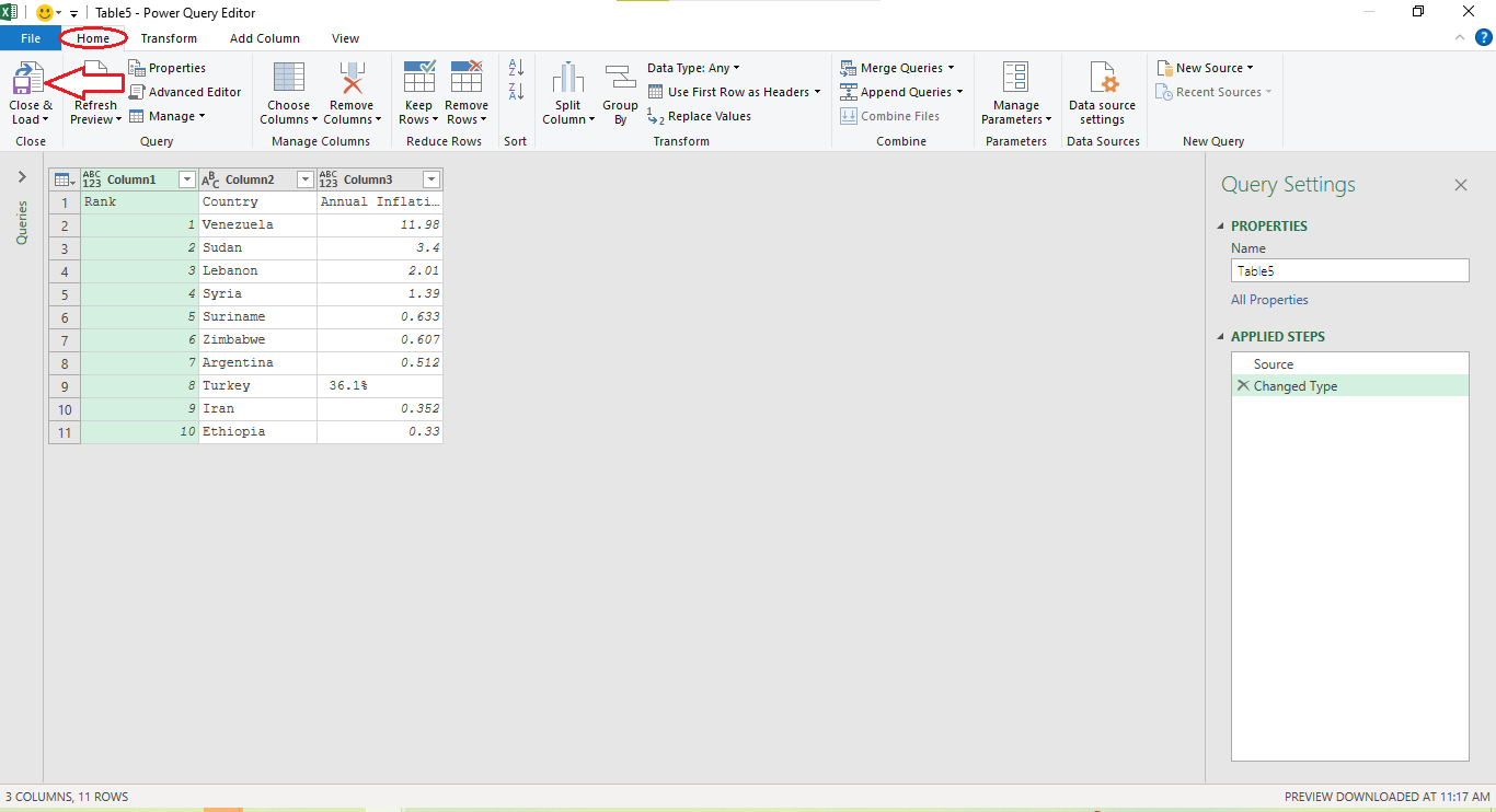
Now, this will open the Power Query Editor, where it loads all the data in. You can maximize the window for better viewing of the data.

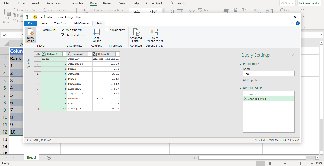
Note: Monospaced is checked here if you prefer a different font style.

Next, you just need to “Close & Load” so you can have a copy of this table.

And then, you will just repeat the process. Go back to “Sheet 1”. Go to the “Data” tab and click “From Table/Range”.

Note: The purpose of repeating the process is just so you can reference the table that you just created.

If you have it noticed, on the left, you can see the “Queries” tab. Click on the arrow to expand it. 

Here, you can see the Table that we have just created. If the formula bar is missing, simply head to the ‘View’ tab and ensure that the Formula bar is checked.

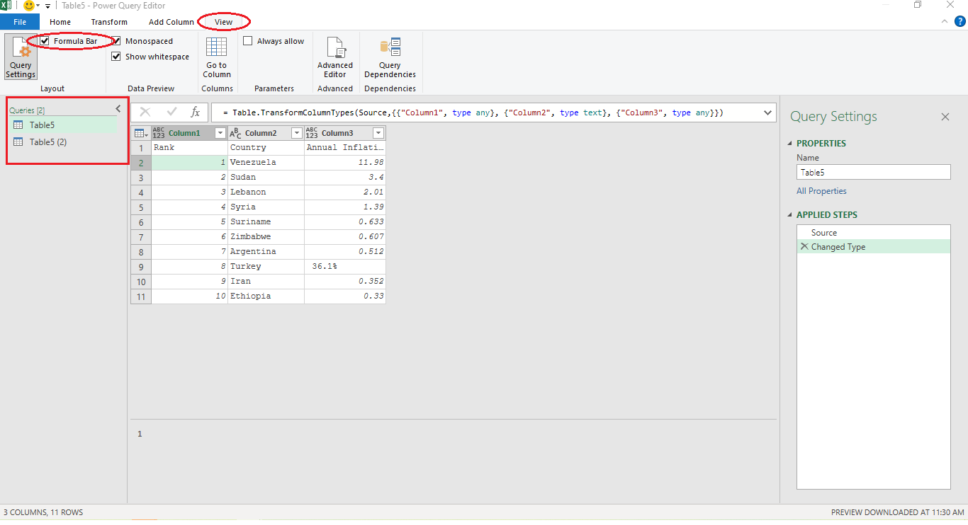
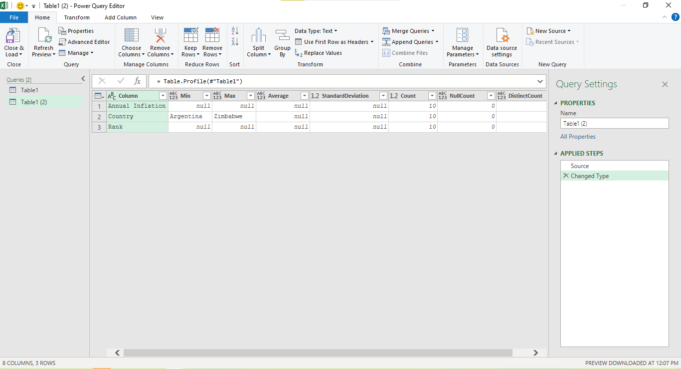
Next, you need to empty the formula bar under Table1 (2) and put there =Table.Profile(#”Table1″)

Note: This is basically to reference Table1. What the query is trying to achieve is just to do a data profile on the data from Table1.

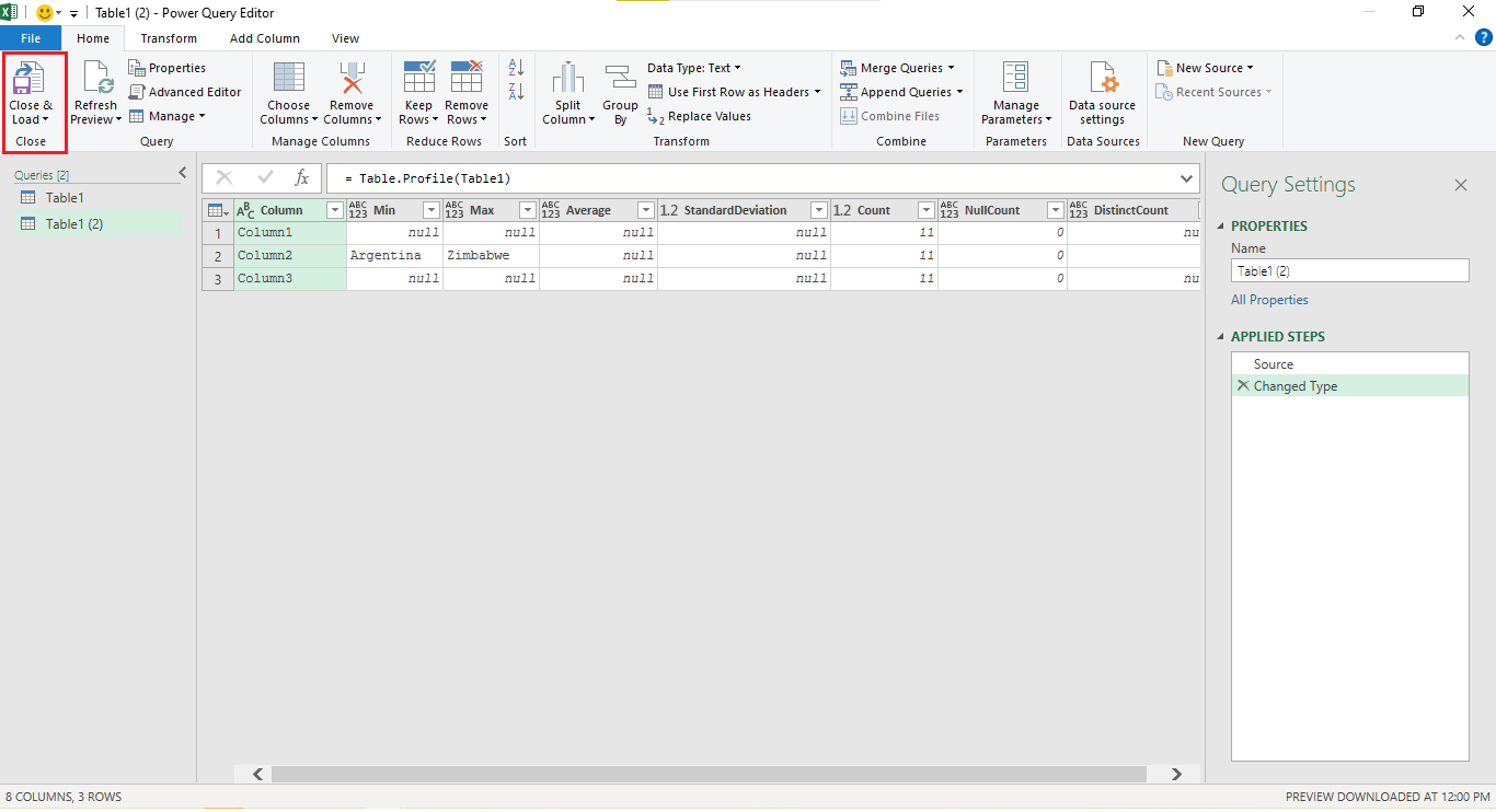
Now that it worked, just go to “Close & Load”.

Step 3: Use Excel Formulas for Basic Data Profiling

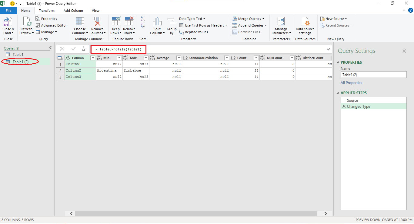
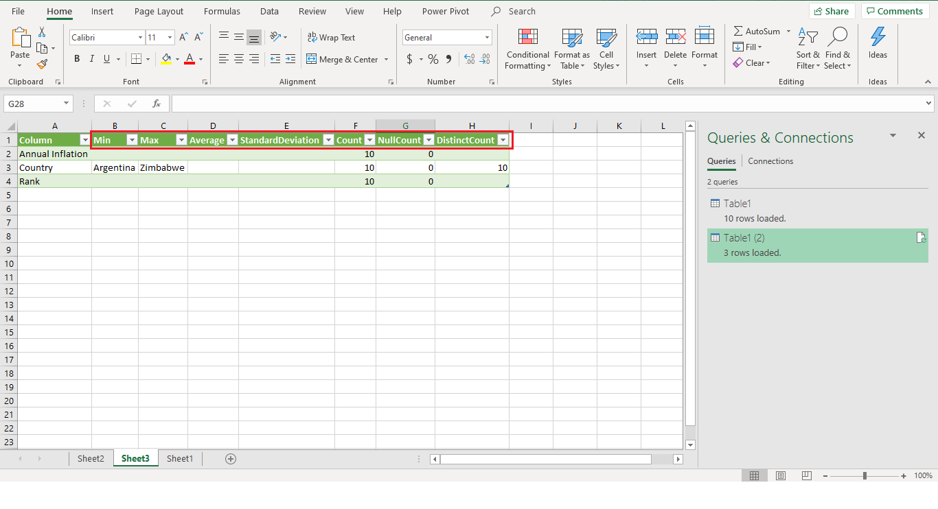
Now all the data has been loaded. Let’s quickly analyze and see what we can find. All of sudden, we can see that it has added new columns based on the initial columns that we have on our Sheet1 (Rank, Country, Annual Inflation). 

The Data Profiling Tool creates these columns.

MIN: This function identifies the minimum value within a specified range of cells. 

MAX: MAX is the counterpart of MIN. It identifies the maximum value within a specified range of cells. 

AVERAGE: This function calculates the arithmetic mean of a range of cells. It adds up all the values in the range and divides the sum by the count of numbers in that range. Calculate the average value using =AVERAGE(range).

MEDIAN: This function returns the median value of a dataset, which is the middle value when the data set is ordered from least to greatest. If the dataset has an odd number of values, the median is the middle value. If the dataset has an even number of values, the median is the average of the two middle values. Find the median value with =MEDIAN(range).

STANDARD DEVIATION: Calculate the standard deviation of a dataset using the formula =STDEV(range). This function measures the amount of variation or dispersion in a set of values.

COUNT: Count the number of cells that contain numbers within a specified range using =COUNT(range). This function returns the count of numeric values in a dataset.

NULLCOUNT: Determine the number of empty or null cells within a range using =COUNTBLANK(range). This function counts the number of cells in a range that are blank.

DISTINCT COUNT: Count the number of unique values in a range with =COUNTUNIQUE(range). This function returns the count of unique values in a dataset, disregarding any duplicates.

Analyzing the types of data you have (e.g., numeric, text) can help in understanding how to treat them in further analysis. Manually inspect columns to determine their data type.

Use =TYPE(cell) to get a number representing the data type in a specific cell (e.g., 1 for numbers, 2 for text).